FIM-Python documentation
Quick Start
Introduction
This library implements the Fast Iterative method that solves the anisotropic eikonal equation on triangulated surfaces, tetrahedral meshes and line networks (equivalent to the Dijkstra’s algorithm in this case), for arbitrary dimensions.
The anisotropic eikonal equation that is solved, is given by the partial differential equation
The library computes \(\phi\) for a given \(D\), \(\mathbf{x}_0\) and \(g\). In practice, this problem is often associated to computing the earliest arrival times \(\phi\) from a set of given starting points \(\mathbf{x}_0\) through a heterogeneous medium (i.e. different velocities are assigned throughout the medium).
Usage
The following shorthand notations are important to know:
\(n\): Number of points
\(m\): Number of elements
\(d\): Dimensionality of the points and metrics (\(D \in \mathbb{R}^{d \times d}\))
\(d_e\): Number of vertices per elements (2, 3 and 4 for lines, triangles and tetrahedra respectively)
\(k\): Number of discrete points \(\mathbf{x}_0 \in \Gamma\) and respective values in \(g(\mathbf{x}_0)\)
\(M := D^{-1}\): The actual metric used in all computations. This is is computed internally and automatically by the library (no need for you to invert \(D\))
precision: The chosen precision for the solver at the initialization
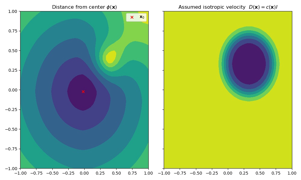
This example computes the solution to the anisotropic eikonal equation for a simple square domain \(\Omega = [-1, 1]^2\), with \(n = 50^2, d = 2, d_e = 3\) and a given isotropic \(D\). This example requires additionally matplotlib and scipy.
import numpy as np
import cupy as cp
from fimpy.solver import FIMPY
from scipy.spatial import Delaunay
import matplotlib.pyplot as plt

#Create triangulated points in 2D
x = np.linspace(-1, 1, num=50)
X, Y = np.meshgrid(x, x)
points = np.stack([X, Y], axis=-1).reshape([-1, 2]).astype(np.float32)
elems = Delaunay(points).simplices
elem_centers = np.mean(points[elems], axis=1)

#The domain will have a small spot where movement will be slow
velocity_f = lambda x: (1 / (1 + np.exp(3.5 - 25*np.linalg.norm(x - np.array([[0.33, 0.33]]), axis=-1)**2)))
velocity_p = velocity_f(points) #For plotting
velocity_e = velocity_f(elem_centers) #For computing
D = np.eye(2, dtype=np.float32)[np.newaxis] * velocity_e[..., np.newaxis, np.newaxis] #Isotropic propagation

x0 = np.array([np.argmin(np.linalg.norm(points, axis=-1), axis=0)])
x0_vals = np.array([0.])

#Create a FIM solver, by default the GPU solver will be called with the active list
#Set device='cpu' to run on cpu and use_active_list=false to use Jacobi method
fim = FIMPY.create_fim_solver(points, elems, D)
phi = fim.comp_fim(x0, x0_vals)

#Plot the data of all points to the given x0 at the center of the domain
fig, axes = plt.subplots(nrows=1, ncols=2, sharey=True)
cont_f1 = axes[0].contourf(X, Y, phi.get().reshape(X.shape))
axes[0].set_title("Distance from center")

cont_f2 = axes[1].contourf(X, Y, velocity_p.reshape(X.shape))
axes[1].set_title("Assumed isotropic velocity")
plt.show()
You should see the following figure with the computed \(\phi\) for the given \(D = c I\).
Installation
To install, either clone the repository and install it:
git clone https://github.com/thomgrand/fim-python .
pip install -e .[gpu]
or simply install the library over PyPI.
pip install fim-python[gpu]
Note
Installing the GPU version might take a while since many cupy modules are compiled using your system’s nvcc compiler.
You can install the cupy binaries first as mentioned here, before installing fimpy.